Customer churn is a critical challenge for businesses seeking long-term customer relationships. In this project our goal is to:
Predict churn: Identify which customers are most likely to exit.
Extract insights: Understand the key drivers of churn.
Develop practical recommendations: Offer actionable strategies to reduce churn.
We build and evaluate several predictive models and then derive business insights from feature importance analysis—all without resampling the dataset.
Dataset Details
The customer churn dataset includes a mix of demographic, financial, and behavioral variables. Below is a detailed description of each feature:
RowNumber: A sequential number assigned to each record. This serves solely as an index and does not hold predictive value.
CustomerId: A unique identifier for each customer. While useful for record keeping, it is not used for modeling.
Surname: The last name of the customer. This variable is not predictive and is excluded from the analysis.
CreditScore: A numerical score representing the customer’s credit rating. Lower credit scores typically indicate higher financial risk, which may correlate with churn.
Geography: The country where the customer is based (e.g., France, Spain, Germany). This categorical variable might capture regional economic and cultural differences affecting churn.
Gender: The customer’s gender, recorded as "male" or "female." Gender differences can influence customer behavior patterns.
Age: The customer’s age in years. Age is a critical factor, as life stage and financial needs evolve over time.
Tenure: The number of years the customer has been with the service provider. Longer tenure might imply stronger relationships, although it may also indicate potential complacency.
Balance: The account balance of the customer. Extremes in balance, either very high or very low, may be indicative of risk.
NumOfProducts: The number of products or services that the customer is using. Customers with more products might be less likely to churn.
HasCrCard: A binary indicator showing whether the customer holds a credit card (0 = no, 1 = yes).
IsActiveMember: A binary variable indicating whether the customer is an active member of the service (0 = inactive, 1 = active).
EstimatedSalary: The customer’s estimated annual salary. This financial indicator can correlate with spending power and loyalty.
Exited: The target variable, where 1 indicates that the customer left (churned) and 0 indicates that they stayed.
Data Loading and Exploration
In this section we load the customer churn dataset and perform initial exploratory analysis.
library(readr)library(dplyr)
Attaching package: 'dplyr'
The following objects are masked from 'package:stats':

    filter, lag
The following objects are masked from 'package:base':

    intersect, setdiff, setequal, union
library(ggplot2)library(caret)
Loading required package: lattice
# Load the datasetdf <-read.csv("churn.csv", stringsAsFactors =FALSE)# Overview of the dataset structure and summary statisticssummary(df)
   RowNumber       CustomerId         Surname           CreditScore
 Min.   :    1   Min.   :15565701   Length:10000       Min.   :350.0
 1st Qu.: 2501   1st Qu.:15628528   Class :character   1st Qu.:584.0
 Median : 5000   Median :15690738   Mode  :character   Median :652.0
 Mean   : 5000   Mean   :15690941                      Mean   :650.5
 3rd Qu.: 7500   3rd Qu.:15753234                      3rd Qu.:718.0
 Max.   :10000   Max.   :15815690                      Max.   :850.0
  Geography            Gender               Age            Tenure
 Length:10000       Length:10000       Min.   :18.00   Min.   : 0.000
 Class :character   Class :character   1st Qu.:32.00   1st Qu.: 3.000
 Mode  :character   Mode  :character   Median :37.00   Median : 5.000
                                       Mean   :38.92   Mean   : 5.013
                                       3rd Qu.:44.00   3rd Qu.: 7.000
                                       Max.   :92.00   Max.   :10.000
    Balance       NumOfProducts    HasCrCard      IsActiveMember
 Min.   :     0   Min.   :1.00   Min.   :0.0000   Min.   :0.0000
 1st Qu.:     0   1st Qu.:1.00   1st Qu.:0.0000   1st Qu.:0.0000
 Median : 97199   Median :1.00   Median :1.0000   Median :1.0000
 Mean   : 76486   Mean   :1.53   Mean   :0.7055   Mean   :0.5151
 3rd Qu.:127644   3rd Qu.:2.00   3rd Qu.:1.0000   3rd Qu.:1.0000
 Max.   :250898   Max.   :4.00   Max.   :1.0000   Max.   :1.0000
 EstimatedSalary         Exited
 Min.   :    11.58   Min.   :0.0000
 1st Qu.: 51002.11   1st Qu.:0.0000
 Median :100193.91   Median :0.0000
 Mean   :100090.24   Mean   :0.2037
 3rd Qu.:149388.25   3rd Qu.:0.0000
 Max.   :199992.48   Max.   :1.0000
Exploratory Visualizations
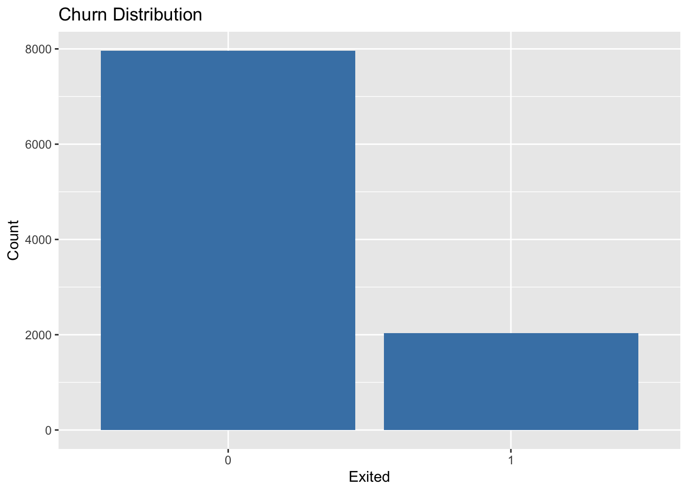
Visualizations help us understand key variables and the distribution of churn in our data.
# Churn distributionggplot(df, aes(x =factor(Exited))) +geom_bar(fill ="steelblue") +labs(title ="Churn Distribution", x ="Exited", y ="Count")
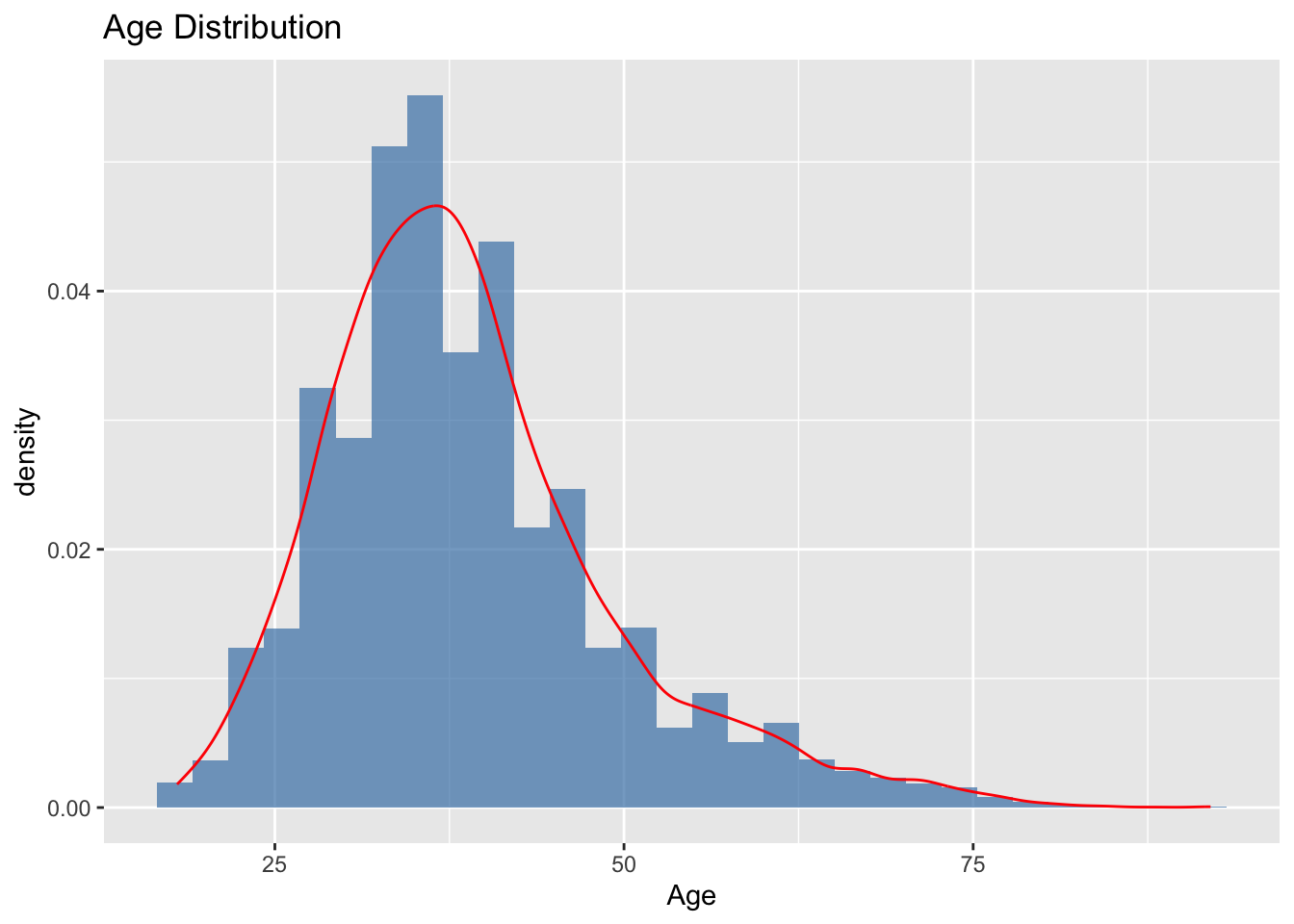
# Age distribution with density curveggplot(df, aes(x = Age)) +geom_histogram(aes(y = ..density..), bins =30, fill ="steelblue", alpha =0.7) +geom_density(color ="red") +labs(title ="Age Distribution")
Warning: The dot-dot notation (`..density..`) was deprecated in ggplot2 3.4.0.
ℹ Please use `after_stat(density)` instead.
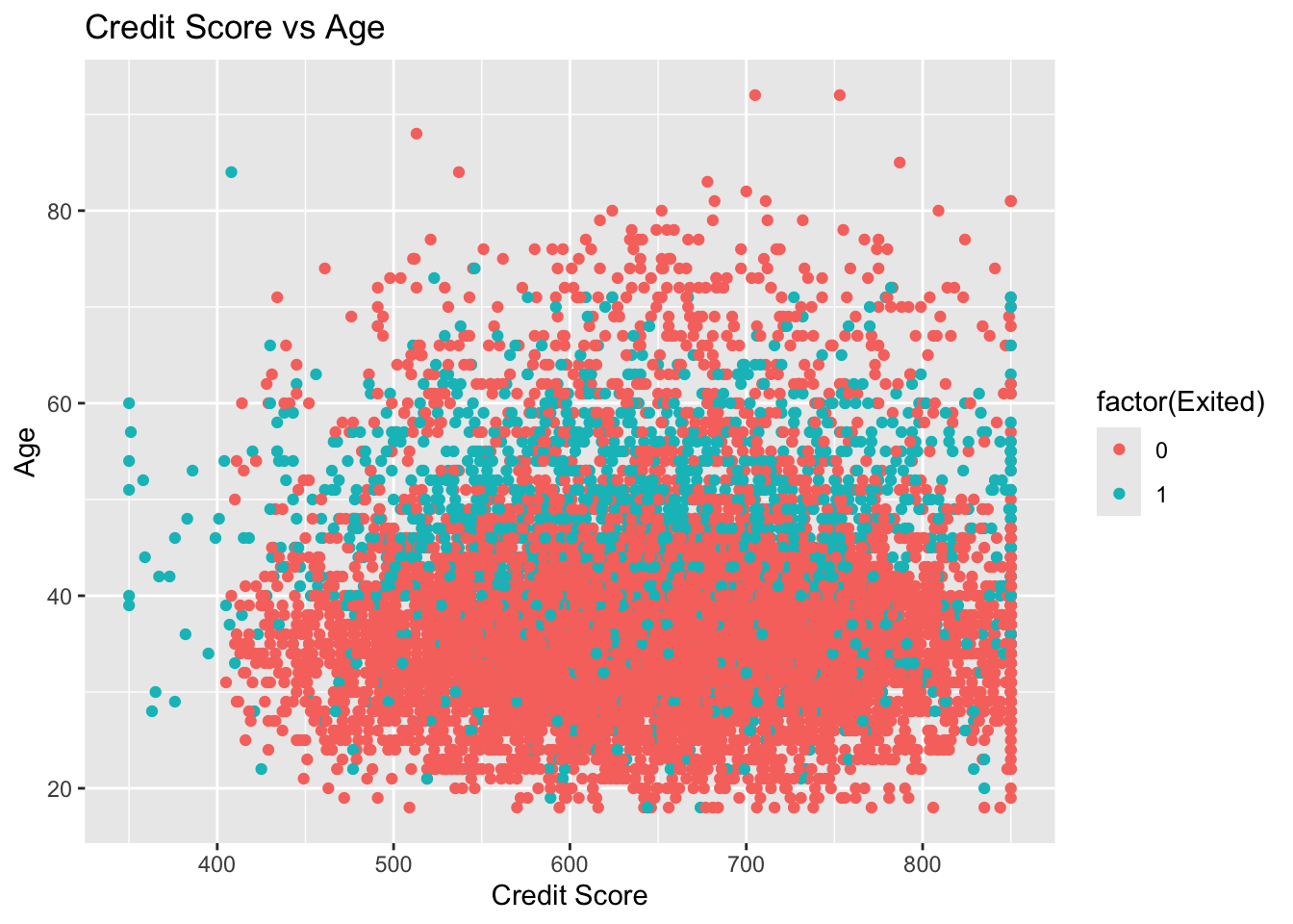
# Scatter plot: Credit Score vs Age (colored by churn)ggplot(df, aes(x = CreditScore, y = Age, color =factor(Exited))) +geom_point() +labs(title ="Credit Score vs Age", x ="Credit Score", y ="Age")
Data Preprocessing and Feature Engineering
The raw data contains variables that are not directly useful for modeling; this section focuses on cleaning and enhancing our features. I begin by removing non-predictive columns such as customer identifiers and handle missing values to ensure consistency. Next, one-hot encoding is applied to transform categorical variables into a suitable numerical format. Further, we develop new features such as Customer Lifetime Value (CLV), AgeGroup, and the Tenure-Age Ratio. These engineered features capture additional nuances—from a customer’s financial engagement to their loyalty—ultimately providing a richer dataset for predictive modeling.
# Separate target variable and predictorstarget <- df$Exitedfeatures <- df %>% dplyr::select(-Exited)# Remove non-predictive columnsfeatures <- features %>% dplyr::select(-RowNumber, -CustomerId, -Surname)# Remove rows with missing valuesfeatures <-na.omit(features)target <- target[as.numeric(rownames(features))]# One-hot encoding for categorical variables ('Geography' and 'Gender')dummy_model <-dummyVars(" ~ .", data = features, fullRank =TRUE)features <-data.frame(predict(dummy_model, newdata = features))# Feature Engineering# Create a measure of Customer Lifetime Value (CLV)if("EstimatedSalary"%in%names(df) &"Balance"%in%names(df)){ features$CLV <- df$EstimatedSalary * df$Balance /100000}# Create an AgeGroup variablefeatures$AgeGroup <-cut(df$Age,breaks =c(0, 30, 45, 60, 100),labels =c("Young", "MiddleAged", "Senior", "Elderly"))# Create a Tenure-Age Ratio featureif("Tenure"%in%names(df) &"Age"%in%names(df)){ features$TenureAgeRatio <- df$Tenure / df$Age}# Reapply one-hot encoding after adding new categorical featuresdummy_model_fe <-dummyVars(" ~ .", data = features, fullRank =TRUE)features <-data.frame(predict(dummy_model_fe, newdata = features))
Splitting and Scaling Data
In this section, I partition the dataset (using a 70/30 split) and then standardize the predictor variables to eliminate scale differences.
set.seed(42)trainIndex <-createDataPartition(target, p =0.7, list =FALSE)x_train <- features[trainIndex, ]x_test <- features[-trainIndex, ]y_train <- target[trainIndex]y_test <- target[-trainIndex]# Scale the datapreProcValues <-preProcess(x_train, method =c("center", "scale"))x_train_scaled <-predict(preProcValues, x_train)x_test_scaled <-predict(preProcValues, x_test)
Modeling and Evaluation
Next, we build several predictive models to assess which best identifies churn (class 1). Our strategy involves training models such as Logistic Regression, Decision Tree, Random Forest, SVM, and KNN. The focus is on capturing churn accurately to support targeted retention initiatives.
library(xgboost)
Attaching package: 'xgboost'
The following object is masked from 'package:dplyr':

    slice
library(rpart)library(randomForest)
randomForest 4.7-1.2
Type rfNews() to see new features/changes/bug fixes.
Attaching package: 'randomForest'
The following object is masked from 'package:ggplot2':

    margin
The following object is masked from 'package:dplyr':

    combine
library(e1071)library(naivebayes)
naivebayes 1.0.0 loaded
For more information please visit:
https://majkamichal.github.io/naivebayes/
library(MASS)
Attaching package: 'MASS'
The following object is masked from 'package:dplyr':

    select
evaluate_model <-function(model_func, train_data, test_data, train_labels, test_labels, ...) {# Train the model using the supplied function model_fit <-model_func(train_data, train_labels, ...)# Generate predictions predictions <-predict(model_fit, test_data)if (inherits(model_fit, "glm")) {# For logistic regression, convert probabilities to binary labels predictions <-ifelse(predictions >0.5, 1, 0) }# Calculate accuracy and print confusion matrix acc <-mean(predictions == test_labels)cat("Accuracy:", round(acc, 4), "\n") cm <-confusionMatrix(as.factor(predictions), as.factor(test_labels))print(cm)return(model_fit)}
Model Training Functions
Below are sample functions for training four different models: Logistic Regression, Decision Tree, Random Forest, and KNN.
# Logistic Regressionlr_model_func <-function(x, y, ...) { data <-cbind(x, Exited = y)glm(Exited ~ ., data = data, family = binomial)}# Decision Treedt_model_func <-function(x, y, ...) { data <-cbind(x, Exited =as.factor(y))rpart(Exited ~ ., data = data, method ="class")}# Random Forestrf_model_func <-function(x, y, ...) { data <-cbind(x, Exited =as.factor(y))randomForest(Exited ~ ., data = data, ...)}# Support Vector Machine (SVM)svm_model_func <-function(x, y, ...) { data <-cbind(x, Exited =as.factor(y))svm(Exited ~ ., data = data, probability =TRUE, ...)}# k-Nearest Neighbors (KNN) using caret for reproducibilityknn_model_func <-function(x, y, k =5, ...) { data <-cbind(x, Exited =as.factor(y))train(Exited ~ ., data = data, method ="knn",tuneGrid =data.frame(k = k),trControl =trainControl(method ="none"))}
Baseline Model Training and Evaluation
Using the model evaluation utility, we train and compare several baseline models to see which one most accurately predicts churn, especially focusing on recall for the churn class (class 1).
Accuracy: 0.855
Confusion Matrix and Statistics

          Reference
Prediction    0    1
         0 2317  368
         1   67  248

               Accuracy : 0.855
                 95% CI : (0.8419, 0.8674)
    No Information Rate : 0.7947
    P-Value [Acc > NIR] : < 2.2e-16

                  Kappa : 0.4574

 Mcnemar's Test P-Value : < 2.2e-16

            Sensitivity : 0.9719
            Specificity : 0.4026
         Pos Pred Value : 0.8629
         Neg Pred Value : 0.7873
             Prevalence : 0.7947
         Detection Rate : 0.7723
   Detection Prevalence : 0.8950
      Balanced Accuracy : 0.6872

       'Positive' Class : 0
cat("### k-Nearest Neighbors (KNN)\n")
### k-Nearest Neighbors (KNN)
knn_model <-evaluate_model(knn_model_func, x_train_scaled, x_test_scaled, y_train, y_test, k =5)
Accuracy: 0.8273
Confusion Matrix and Statistics

          Reference
Prediction    0    1
         0 2249  383
         1  135  233

               Accuracy : 0.8273
                 95% CI : (0.8133, 0.8407)
    No Information Rate : 0.7947
    P-Value [Acc > NIR] : 3.469e-06

                  Kappa : 0.3781

 Mcnemar's Test P-Value : < 2.2e-16

            Sensitivity : 0.9434
            Specificity : 0.3782
         Pos Pred Value : 0.8545
         Neg Pred Value : 0.6332
             Prevalence : 0.7947
         Detection Rate : 0.7497
   Detection Prevalence : 0.8773
      Balanced Accuracy : 0.6608

       'Positive' Class : 0
In our baseline evaluations, the Random Forest model emerged as the most promising candidate for accurately predicting churn. This model not only demonstrated higher overall accuracy and balanced performance compared to alternatives such as logistic regression, SVM, and KNN, but it also delivered superior sensitivity towards class 1 (churners), which is critical for targeted retention strategies.
Feature Importance and Business Insights
Understanding the key drivers of churn is critical to developing actionable business strategies. In this phase, we focus on a cost-sensitive Random Forest model—chosen for its superior performance in identifying churners—by assigning a higher weight to class 1. This approach reduces the misclassification error for the minority class and highlights the most influential features.
rf_train <-cbind(x_train_scaled, Exited =factor(y_train))# Train a cost-sensitive Random Forest model.# Here, we assign a higher weight to class "1" (churn) to encourage the model to better identify churn cases.library(randomForest)rf_cs <-randomForest(Exited ~ ., data = rf_train,ntree =100,classwt =c("0"=1, "1"=8))# Display model summaryprint(rf_cs)
Call:
 randomForest(formula = Exited ~ ., data = rf_train, ntree = 100,      classwt = c(`0` = 1, `1` = 8))
               Type of random forest: classification
                     Number of trees: 100
No. of variables tried at each split: 4

        OOB estimate of  error rate: 14.76%
Confusion matrix:
     0   1 class.error
0 5329 250   0.0448109
1  783 638   0.5510204
# Extract feature importance metrics and visualize them.importance_rf <-importance(rf_cs)print(importance_rf)
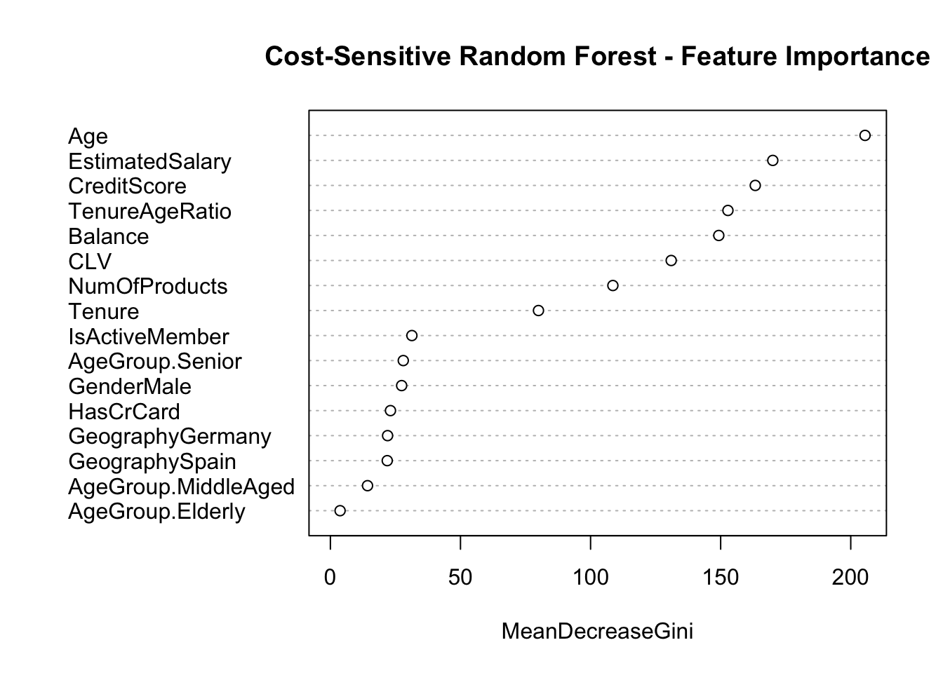
varImpPlot(rf_cs, main ="Cost-Sensitive Random Forest - Feature Importance")
The feature importance results reveal that financial indicators such as Credit Score, Balance, and the engineered Customer Lifetime Value (CLV) are key drivers of churn. In addition, engagement indicators like the Tenure-Age Ratio and demographic segmentation via Age Group provide further insights into customer behavior. These findings enable the business to target intervention strategies more precisely—focusing on customers who exhibit financial stress or low engagement.
Conclusion and Next Steps
In this project, we developed a cost-sensitive Random Forest model to predict customer churn while specifically focusing on reducing the misclassification error for churners (class 1). By incorporating advanced feature engineering—such as leveraging financial indicators (Credit Score, Balance), Customer Lifetime Value (CLV), and engagement metrics (Tenure-Age Ratio, Age Group)—we obtained actionable insights into the drivers of customer churn.
Key Findings:
Model Performance: The cost-sensitive Random Forest model has been tuned to emphasize the detection of churners, achieving improved sensitivity while accepting a trade-off in specificity. Our analysis identified that, despite an overall strong performance, misclassification for class 1 remained a challenge. Adjustments such as threshold tuning provide a practical approach to further enhance the detection of at-risk customers.
Feature Importance:
Variables such as Credit Score, Balance, CLV, and Tenure-Age Ratio emerged as the most influential factors. These results confirm that financial stress and engagement-related features are critical in predicting churn, thereby pinpointing specific customer segments where retention efforts could be most beneficial.
Business Implications:
The insights gained from the model directly inform targeted retention strategies:
Tailored Interventions: Customers with low Credit Scores and high Balances should be prioritized for personalized offers such as payment flexibility or financial counseling.
Segmented Engagement: Distinct communication strategies should be designed for different demographic groups, as highlighted by the importance of Age Group and Tenure-Age Ratio.
Operational Integration: Implementing the model within the company’s CRM system will allow continuous monitoring of churn risk, enabling proactive and data-driven retention campaigns.
Next Steps:
Refinement of Thresholds and Cost Settings:
Experiment further with threshold adjustments and class weight settings to optimize the balance between sensitivity and specificity. Continuous calibration will help reduce the error rate for churners without excessively increasing false positives.
Integration into Business Processes:
Work collaboratively with the marketing and customer service teams to integrate the predictive model into the CRM. This integration should include an automated alert system that identifies and flags high-risk customers, ensuring timely intervention.
Monitoring and Feedback Loop:
Establish a regular review mechanism to monitor the model’s performance in real-world settings. Use this feedback to fine-tune features and update the model periodically, thereby adapting to evolving customer behaviors and market dynamics.
Exploration of Additional Data Sources:
Consider incorporating additional data—such as customer engagement metrics from digital interactions or feedback scores—to further enhance the model’s predictive power and provide a deeper understanding of churn drivers.
Final Thoughts
By blending advanced feature engineering with cost-sensitive learning, this project has not only yielded a robust predictive model but also delivered clear, actionable business insights. These insights pave the way for targeted retention strategies that can directly contribute to reducing churn rates and improving customer lifetime value. The ongoing challenge will be to integrate these models into the operational framework and iteratively refine them based on real-time data and business outcomes.